
Andrej Karpathy 的 nanoGPT lecture demo 详解。主要包括学习资料、总结输出、为什么学 nanoGPT、详解 nanoGPT 四个部分。
#! https://zhuanlan.zhihu.com/p/682466360
Andrej Karpathy 的 nanoGPT lecture demo 详解
1. 学习资料
- 大佬 Andrej Karpathy, 李飞飞高徒,前openai研究员,前Tesla AI总监,在youtobe上有一系列的深度学习课程,其中有一节是关于nanoGPT的,
- 全英文 YouToBe: Let’s build GPT: from scratch, in code, spelled out.
- 中英文字幕 哔哩哔哩: Let’s build GPT: from scratch, in code, spelled out.
2. 总结输出
代码详见github:https://github.com/HuZixia/nanoGPT-lecture.git
git代码介绍

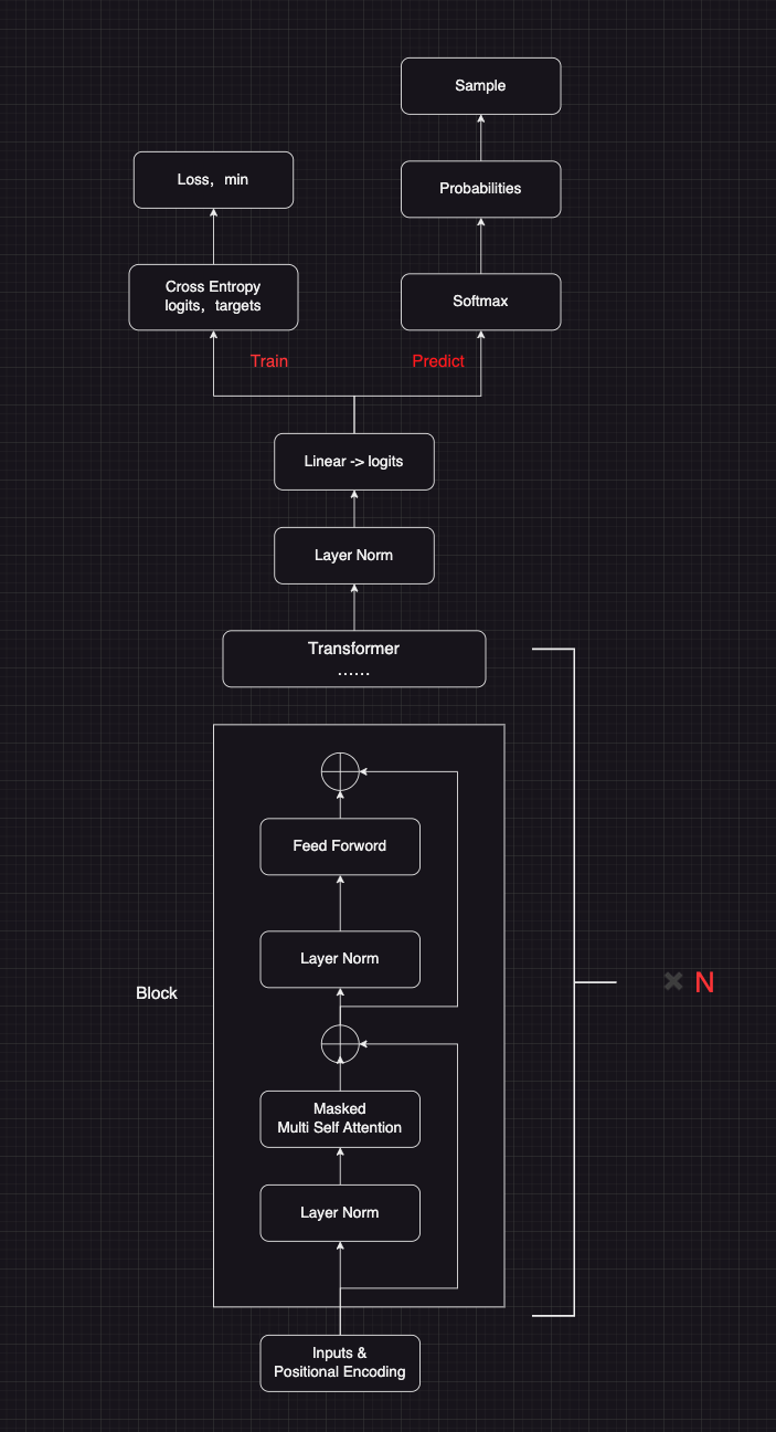
- gpt demo 模型结构
3. 为什么学 nanoGPT
- 小型化和效率化:nanoGPT 是一种小型的 GPT 模型,具有更少的参数,这使得它在资源受限的环境中更加实用。
- 了解 LLM 的实现原理,掌握 PyTorch 和 Transformers 的使用。
- 学习nanoGPT,可以了解GPT模型的工作原理,以及如何实现一个简单的GPT模型。
4. 详解 nanoGPT
- GPT demo 详解
- 本文主要讲解 Let’s build GPT: from scratch, in code, spelled out 视频中的demo,更多的nanoGPT代码,以后有时间分享。
import torch
import torch.nn as nn
from torch.nn import functional as F

# 超参数设置
# hyperparameters
batch_size = 16 # how many independent sequences will we process in parallel?
block_size = 32 # what is the maximum context length for predictions?
max_iters = 5000
eval_interval = 100
learning_rate = 1e-3
device = 'cuda' if torch.cuda.is_available() else 'cpu'
eval_iters = 200
n_embd = 64
n_head = 4
n_layer = 4
dropout = 0.0
# ------------

torch.manual_seed(1337)

# 1. 数据处理
# wget https://raw.githubusercontent.com/karpathy/char-rnn/master/data/tinyshakespeare/input.txt
with open('input.txt', 'r', encoding='utf-8') as f:
    text = f.read()

# here are all the unique characters that occur in this text
chars = sorted(list(set(text)))
vocab_size = len(chars)
# create a mapping from characters to integers
stoi = { ch:i for i,ch in enumerate(chars) }
itos = { i:ch for i,ch in enumerate(chars) }
encode = lambda s: [stoi[c] for c in s] # encoder: take a string, output a list of integers
decode = lambda l: ''.join([itos[i] for i in l]) # decoder: take a list of integers, output a string

# 2. 数据集划分
# Train and test splits
data = torch.tensor(encode(text), dtype=torch.long)
n = int(0.9*len(data)) # first 90% will be train, rest val
train_data = data[:n]
val_data = data[n:]

# 3. 数据分批
# data loading
def get_batch(split):
    # generate a small batch of data of inputs x and targets y
    data = train_data if split == 'train' else val_data
    ix = torch.randint(len(data) - block_size, (batch_size,))
    x = torch.stack([data[i:i+block_size] for i in ix])
    y = torch.stack([data[i+1:i+block_size+1] for i in ix])
    x, y = x.to(device), y.to(device)
    return x, y

# 4. 模型评估
# 评估模型在训练集和验证集上的平均损失。这个函数的实现非常简单:它首先将模型设置为评估模式,然后对每个数据集进行eval_iters次迭代。
# 在每次迭代中,它获取一个小批量数据,然后计算模型的输出和损失。最后,它返回每个数据集的平均损失。
@torch.no_grad()
def estimate_loss():
    out = {}
    model.eval()
    for split in ['train', 'val']:
        losses = torch.zeros(eval_iters)
        for k in range(eval_iters):
            X, Y = get_batch(split)
            logits, loss = model(X, Y)
            losses[k] = loss.item()
        out[split] = losses.mean()
    model.train()
    return out

# 5. 模型head定义
class Head(nn.Module):
    """ one head of self-attention """

    def __init__(self, head_size):
        super().__init__()
        self.key = nn.Linear(n_embd, head_size, bias=False)
        self.query = nn.Linear(n_embd, head_size, bias=False)
        self.value = nn.Linear(n_embd, head_size, bias=False)
        # 创建一个下三角矩阵,并将其注册为模型的一个缓冲区。
        # 这个下三角矩阵将被用作self-attention的权重矩阵,它将确保模型只能在当前时间步之前的时间步上进行自注意力操作。
        self.register_buffer('tril', torch.tril(torch.ones(block_size, block_size)))

        self.dropout = nn.Dropout(dropout)

    def forward(self, x):
        B,T,C = x.shape
        k = self.key(x)   # (B,T,C)
        q = self.query(x) # (B,T,C)
        # compute attention scores ("affinities")
        wei = q @ k.transpose(-2,-1) * C**-0.5 # (B, T, C) @ (B, C, T) -> (B, T, T)
        wei = wei.masked_fill(self.tril[:T, :T] == 0, float('-inf')) # (B, T, T)
        wei = F.softmax(wei, dim=-1) # (B, T, T)
        wei = self.dropout(wei)
        # perform the weighted aggregation of the values
        v = self.value(x) # (B,T,C)
        out = wei @ v # (B, T, T) @ (B, T, C) -> (B, T, C)
        return out

# 6. 模型MultiHeadAttention定义
# 实现多头自注意力机制。在这个机制中,我们并行地进行多次自注意力计算,然后将结果拼接起来,通过一个线性层和一个dropout层进行处理,得到最终的输出。
# 这种方法可以让模型在不同的表示子空间中学习输入的不同特征。
class MultiHeadAttention(nn.Module):
    """ multiple heads of self-attention in parallel """

    # __init__方法是类的构造函数,它接收两个参数:num_heads和head_size。num_heads是注意力头的数量,head_size是每个注意力头的大小。
    # 创建了一个nn.ModuleList,它包含了num_heads个Head对象。我们还定义了一个线性层self.proj和一个dropout层self.dropout。
    def __init__(self, num_heads, head_size):
        super().__init__()
        self.heads = nn.ModuleList([Head(head_size) for _ in range(num_heads)])
        self.proj = nn.Linear(n_embd, n_embd)
        self.dropout = nn.Dropout(dropout)

    # forward方法定义了前向传播的计算过程。首先,我们对每个注意力头h进行计算,然后将结果在最后一个维度上拼接起来,得到out。
    # 然后,我们将out输入到线性层和dropout层,得到最终的输出。
    def forward(self, x):
        out = torch.cat([h(x) for h in self.heads], dim=-1)
        out = self.dropout(self.proj(out))
        return out

# 7. 模型FeedFoward定义
class FeedFoward(nn.Module):
    """ a simple linear layer followed by a non-linearity """

    # 在__init__方法中,我们首先调用了父类的构造函数,然后定义了一个神经网络self.net。这个神经网络是一个nn.Sequential对象,
    # 它包含了两个线性层和一个ReLU激活函数,以及一个dropout层。
    # 第一个线性层将输入的维度扩大到4 * n_embd,然后通过ReLU激活函数进行非线性变换,然后第二个线性层将维度缩小回n_embd,最后通过dropout层进行正则化。
    def __init__(self, n_embd):
        super().__init__()
        self.net = nn.Sequential(
            nn.Linear(n_embd, 4 * n_embd),
            nn.ReLU(),
            nn.Linear(4 * n_embd, n_embd),
            nn.Dropout(dropout),
        )

    def forward(self, x):
        return self.net(x)

# 8. 模型Block定义,layerNorm, multiheadattention, layerNorm, feedforward
# Block类的作用是实现一个Transformer模型中的一个块。这个块包含了一个多头自注意力模块和一个前馈神经网络模块,以及两个层归一化操作。
# 这种结构可以让模型在处理序列数据时,能够同时考虑到每个位置的信息和全局的信息。
class Block(nn.Module):
    """ Transformer block: communication followed by computation """

    def __init__(self, n_embd, n_head):
        # n_embd: embedding dimension, n_head: the number of heads we'd like
        super().__init__()
        head_size = n_embd // n_head
        self.sa = MultiHeadAttention(n_head, head_size)
        self.ffwd = FeedFoward(n_embd)
        self.ln1 = nn.LayerNorm(n_embd)
        self.ln2 = nn.LayerNorm(n_embd)

    # forward方法定义了前向传播的计算过程。首先,我们将输入x进行层归一化,然后输入到自注意力模块中,得到的输出与原始的x相加,得到新的x。
    # 然后,我们将新的x进行层归一化,然后输入到前馈神经网络中,得到的输出与原始的x相加,得到最终的输出。
    def forward(self, x):
        x = x + self.sa(self.ln1(x))
        x = x + self.ffwd(self.ln2(x))
        return x

# 9. 模型BigramLanguageModel定义
# super simple bigram model,训练一个二元语言模型,并生成新的文本。
class BigramLanguageModel(nn.Module):

    def __init__(self):
        super().__init__()
        # each token directly reads off the logits for the next token from a lookup table
        self.token_embedding_table = nn.Embedding(vocab_size, n_embd)
        self.position_embedding_table = nn.Embedding(block_size, n_embd)
        self.blocks = nn.Sequential(*[Block(n_embd, n_head=n_head) for _ in range(n_layer)])
        self.ln_f = nn.LayerNorm(n_embd) # final layer norm
        self.lm_head = nn.Linear(n_embd, vocab_size)

    # forward方法定义了前向传播的计算过程。首先,我们从词嵌入表和位置嵌入表中获取嵌入,然后将它们相加得到x。
    # 然后,我们将x输入到self.blocks中,然后进行层归一化,然后输入到self.lm_head中,得到logits。如果提供了目标,我们会计算交叉熵损失。
    def forward(self, idx, targets=None):
        B, T = idx.shape

        # idx and targets are both (B,T) tensor of integers
        tok_emb = self.token_embedding_table(idx) # (B,T,C)
        pos_emb = self.position_embedding_table(torch.arange(T, device=device)) # (T,C)
        x = tok_emb + pos_emb # (B,T,C)
        x = self.blocks(x) # (B,T,C)
        x = self.ln_f(x) # (B,T,C)
        logits = self.lm_head(x) # (B,T,vocab_size)

        if targets is None:
            loss = None
        else:
            B, T, C = logits.shape
            logits = logits.view(B*T, C)
            targets = targets.view(B*T)
            loss = F.cross_entropy(logits, targets)

        return logits, loss

    # 将当前的索引裁剪到最后的block_size个令牌,然后获取预测的logits,然后只关注最后一个时间步,然后应用softmax得到概率,然后从分布中采样,然后将采样的索引添加到运行的序列中。
    def generate(self, idx, max_new_tokens):
        # idx is (B, T) array of indices in the current context
        for _ in range(max_new_tokens):
            # crop idx to the last block_size tokens
            idx_cond = idx[:, -block_size:]
            # get the predictions
            logits, loss = self(idx_cond)
            # focus only on the last time step
            logits = logits[:, -1, :] # becomes (B, C)
            # apply softmax to get probabilities
            probs = F.softmax(logits, dim=-1) # (B, C)
            # sample from the distribution
            idx_next = torch.multinomial(probs, num_samples=1) # (B, 1)
            # append sampled index to the running sequence
            idx = torch.cat((idx, idx_next), dim=1) # (B, T+1)
        return idx


# 10. 模型实例化
model = BigramLanguageModel()
m = model.to(device)
# print the number of parameters in the model
# 将其移动到设备device上。然后,我们打印出模型中的参数数量。
print(sum(p.numel() for p in m.parameters())/1e6, 'M parameters')

# create a PyTorch optimizer
optimizer = torch.optim.AdamW(model.parameters(), lr=learning_rate)

for iter in range(max_iters):

    # every once in a while evaluate the loss on train and val sets
    if iter % eval_interval == 0 or iter == max_iters - 1:
        losses = estimate_loss()
        print(f"step {iter}: train loss {losses['train']:.4f}, val loss {losses['val']:.4f}")

    # 从训练集中采样一个批次的数据xb和yb,然后将它们输入到模型中,得到logits和loss。然后,我们将优化器的梯度清零,然后计算损失的反向传播,然后更新优化器的参数。
    # 采样一个批次的数据,计算损失,清零梯度,计算反向传播,然后更新参数。这是训练神经网络模型的基本步骤。
    # sample a batch of data
    xb, yb = get_batch('train')

    # evaluate the loss
    logits, loss = model(xb, yb)
    # 清零优化器的梯度。这是因为PyTorch的优化器在每次更新参数时都会累积梯度,所以在每次更新参数之前,我们需要清零梯度。
    optimizer.zero_grad(set_to_none=True)
    # 计算损失的反向传播。这会计算出每个参数的梯度。
    loss.backward()
    # 更新优化器的参数。这会根据每个参数的梯度和学习率来更新参数的值。
    optimizer.step()

# generate from the model
# 用模型来生成新的文本,首先创建一个全零的上下文context,然后将其输入到模型的generate方法中,得到生成的文本,然后将其解码并打印出来。
context = torch.zeros((1, 1), dtype=torch.long, device=device)
print(decode(m.generate(context, max_new_tokens=2000)[0].tolist()))
- 代码执行结果:train loss 和 val loss 变化情况
# 0.209729 M parameters
# step 0: train loss 4.4116, val loss 4.4022
# step 100: train loss 2.6568, val loss 2.6670
# step 200: train loss 2.5091, val loss 2.5059
# step 300: train loss 2.4196, val loss 2.4336
# step 400: train loss 2.3498, val loss 2.3560
# step 500: train loss 2.2964, val loss 2.3130
# step 600: train loss 2.2406, val loss 2.2497
# step 700: train loss 2.2052, val loss 2.2185
# step 800: train loss 2.1633, val loss 2.1861
# step 900: train loss 2.1246, val loss 2.1511
# step 1000: train loss 2.1036, val loss 2.1309
# step 1100: train loss 2.0709, val loss 2.1196
# step 1200: train loss 2.0381, val loss 2.0794
# step 1300: train loss 2.0243, val loss 2.0633
# step 1400: train loss 1.9929, val loss 2.0362
# step 1500: train loss 1.9711, val loss 2.0313
# step 1600: train loss 1.9633, val loss 2.0484
# step 1700: train loss 1.9410, val loss 2.0126
# step 1800: train loss 1.9111, val loss 1.9973
# step 1900: train loss 1.9103, val loss 1.9877
# step 2000: train loss 1.8853, val loss 1.9945
# step 2100: train loss 1.8711, val loss 1.9765
# step 2200: train loss 1.8594, val loss 1.9612
# step 2300: train loss 1.8541, val loss 1.9503
# step 2400: train loss 1.8437, val loss 1.9446
# step 2500: train loss 1.8157, val loss 1.9425
# step 2600: train loss 1.8264, val loss 1.9394
# step 2700: train loss 1.8099, val loss 1.9330
# step 2800: train loss 1.8071, val loss 1.9250
# step 2900: train loss 1.8077, val loss 1.9323
# step 3000: train loss 1.7989, val loss 1.9207
# step 3100: train loss 1.7713, val loss 1.9230
# step 3200: train loss 1.7555, val loss 1.9141
# step 3300: train loss 1.7606, val loss 1.9092
# step 3400: train loss 1.7565, val loss 1.8923
# step 3500: train loss 1.7361, val loss 1.8905
# step 3600: train loss 1.7256, val loss 1.8840
# step 3700: train loss 1.7323, val loss 1.8863
# step 3800: train loss 1.7229, val loss 1.8916
# step 3900: train loss 1.7187, val loss 1.8654
# step 4000: train loss 1.7119, val loss 1.8552
# step 4100: train loss 1.7118, val loss 1.8778
# step 4200: train loss 1.7038, val loss 1.8559
# step 4300: train loss 1.6976, val loss 1.8423
# step 4400: train loss 1.7050, val loss 1.8618
# step 4500: train loss 1.6898, val loss 1.8519
# step 4600: train loss 1.6872, val loss 1.8321
# step 4700: train loss 1.6819, val loss 1.8385
# step 4800: train loss 1.6678, val loss 1.8449
# step 4900: train loss 1.6703, val loss 1.8382
# step 4999: train loss 1.6633, val loss 1.8223
#
# Flie?
#
# WARICENTIO:
# Shrungst bewiter are a toom here:
# In if the wouIes?
# Out; and sate, and for one that I are and those it;
# Git.
#
# WARIO:
# Advory's toble sear; the, will God
# of breath what Mear;
# Was can is your name Burry eyree facge
# For will dath thee herp too thy laments
# That would may clood, one these do spost I vour have weret, where sup.
# How sens Gortunt, which what fit,
# Out thre, is wwife that broth. Who', betch'd your.
#
# TRABELLANE:
# Shall
# My sworn must he anour,
# Buntius; in So metter those make me,
# And fliems, my chince.
#
# POMY:
# Yet my nourtwarly to be thrany's discont,
# If day a gends pmenaton him, say.
#
# DUKE OF YORK:
# The twerefory well streage was babolantand now thing:
# O, this to set myself, cour bid to shall her speesen he crown.
# Vnow as thou thront, plarter no adds in thyself croath.
# My lord, but terruly friend
# Ristomfurts to-mries
# Againt serviet, contandy that kisspy grave, we mine!
# Or he him my spast,
# I so unsinced, wen is bese zable gity;
# Not do to seing, then thee from whosame noby.
# Go and neer thou would may night.
#
# RUCHERSIO:
# That, by tongue will be in him our sitittion;
# She now to be, all goots stespers
# in An rentry. Towe pas-dayfull keep,
# That thy will your sould in him,
# And ladditlebaning that gentrand, which myself, betish end alwied's boy exides'd.
#
# ISABTH:
# My master the slands you great? I shalk;
# Stat the kngscanty on straight boys hitger;
# Becompely his doath; of us Voly.
#
# Sensure:
# And there your worts, all, save infict is a those astold
# of by my felling wit-be in his in
# Hard's deaths chanting me them is seedder'd was busweet.
#
# CORINIUS:
# No, for I have your merch'mord.
# Is you graXut affinzy houth this sele yourders?
#
# POLFORD NORWARD YOMIUS:
# You come you.
#
# POYCUS:
# Thy gleist the dongsorn:
# Nay fantle Becoleforfact tell servy inters! in I know tould lappread
# Goat you sucalf me wars non your
# art:
# As one thumself, who live requann.
# Anjury thee that with, and we not?
# Good the preasurs, comison toOH!
#
# Second Affordmn:-now.
#
# Must wear I pearince?
# And think
关于Masked Multi Self Attention 中的mask的原理和实现:
The mathematical trick in self-attention
- version 1: for loop and gather, use torch.mean
- version 2: using matrix multiply for a weighted aggregation
- version 3: use Softmax
- version 4: self-attention!
详细的讲解和代码,见github:https://github.com/HuZixia/nanoGPT-lecture/blob/main/gpt_dev.ipynb
关于transformer结构,详见 Transformer & 预训练
文档信息
- 本文作者:huzixia
- 本文链接:https://huzixia.github.io/2024/02/16/nanoGPT/
- 版权声明:自由转载-非商用-非衍生-保持署名(创意共享3.0许可证)